Assimilation of Illinois Soil Moisture Data into a Simple Water Balance Model

Gopi Goteti, Amy L. Sansone, Kyle Comanor and Dennis P. Lettenmaier

Department of Civil and Environmental Engineering, Box 352700, University of Washington, Seattle, WA 98195

Overview

Data assimilation methods have been widely used to update atmospheric model estimates of spatially distributed state variables as new observations become available. In the hydrologic sciences analogous problems exist, particularly where observations of soil moisture, the state variable that controls land surface moisture fluxes, are available. We assessed the performance of several data assimilation techniques using the Simple Water Balance (SWB) model of Schaake et al (1996) using soil moisture data for the state of Illinois. Model forcings were derived from gridded precipitation and temperature data produced as part of the Land Data Assimilation System (LDAS) project (Mitchell et al, 1999) for the central U.S. The SWB model was applied over the state of Illinois at ½ degree spatial resolution. Calibration of the model was based on total monthly runoff as compared to one USGS gage. Soil moisture data were assimilated using direct insertion, statistical correction, Newtonian nudging with gridded analysis and Newtonian nudging to individual observations, as defined by Houser et al (1998). In general, the predicted runoff with no assimilation more closely matched the observed runoff using any of the assimilation methods when observed soil moisture was used directly in the assimilation algorithms. This failure to improve runoff predictions was traced to differences in the model-predicted and observed soil moistures. When the mean differences were accounted for, modest improvements in prediction accuracy were achieved relative to the no-assimilation case. Improvements were generally greatest in the spring and summer, and least in the fall and winter.

Project Setting

The Illinois River (figure 1) is a tributary to the Mississippi, and drains most of the northern part of the state of Illinois (approximately 25,000 square miles). It flows generally west across the state until it reaches approximately 89.5° W, where it turns abruptly south to join the Mississippi River. To enable calibration of the model, only the portion upstream of the United States Geological Survey (USGS) gage at Kingston Mines, Il (05568500) was considered. The drainage area above this gage is 15,818 square miles.

Data Description

Model Forcing Data

•Precipitation was derived from gridded precipitation and temperature data produced as part of the Land Data Assimilation System (LDAS) project for the central U.S. by Maurer et al (2000). Snow accumulation and melt were derived from VIC model runs by Maurer et al (2000).

•Potential evapotranspiration was calculated as pan evaporation (Linsley, et al. 1982) according to:

where the vapor pressure deficit (e_s-e_a) = f(T_avg, T_dew as T_min) and v_p is daily wind movement.

Soil Moisture Data

•Soil moisture water equivalent data for 17 stations were obtained from the Global Soil Moisture Data Bank (Robock et al., 2000) and summed over a 2 meter depth.

•For the direct insertion, gridded nudging, and statistical correction assimilation techniques the data were interpolated to a grid using an inverse distance algorithm.

•There were a total of 173 representative days with soil moisture observations over the period from January 1, 1986 through December 31, 1996.

•A representative day was defined as a day for which no more than five stations failed to report either on that day or the two previous or two succeeding days. Missing data are interpolated using an inverse distance weighting scheme

• The soil moisture data are normalized for use in the model as follows

where w_{oberv,wilting,fieldcap} is at the observed, field capacity and wilting point moisture content.

Simple Water Balance (SWB) Model

(See Shaake et al. (1996) for details)

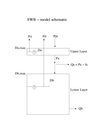
The model has two layers, with upper layer storage (u) representing interception and depression storage, and lower layer storage (b) representing the root zone (figure 2).

Governing equations (in terms of moisture deficits expressed as depths):
Upper and lower layers, respectively:

Evapotranspiration:

where D_u,b are upper and lower layer water deficits, E_u,b is upper and lower layer evaporation. P is precipitation, P_x is excess precipitation, Q_s,g are surface and sub-surface runoff, respectively and E_pb = E_p-E_uwhere E_p is potential evapotranspiration.

No routing of runoff was performed. Instead, a relatively long time period (one month) was selected so that routing effects are minimal.

Runoff generation:

where S_max is a deficit threshold and K_dt is a constant, and Q_max is the maximum possible runoff.

Calibration and Validation

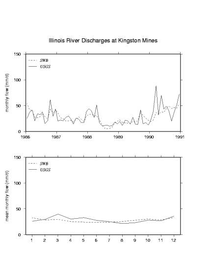
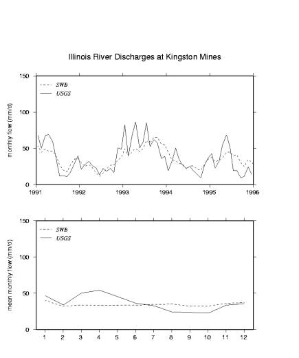
The model was calibrated using mean monthly flow from 1986-1990 (figure 3), and validated for 1991-1995 (figure 4). Calibration was good in a mean monthly sense due in part to the weak seasonal cycle for 86-90. Validation was fair and did not capture the mean monthly seasonal cycle.

DATA ASSIMILATION TECHNIQUES
(see Houser et al. (1998) for a more detailed description of the techniques)

Direct Insertion

•Assumes the observations are perfect

•Replaces the model prediction with the observation when available

Statistical Correction

•Assumes the statistics of the observations are perfect

•Adjusts model standard deviation to the observed

for all i

•Then adjusts the new mean to the observed mean

for all i

Newtonian Nudging with Gridded Analysis

•Nudges model towards observations rather than replacing state variable.

Correction is proportional to difference between modelled and observed states

•Requires observations on regular grid

•

with model forcing term F, weighting term W_¸, data quality factor µ_¸, gain term G_¸, gridded observation ¸_o’, model state ¸. W_¸ and µ_¸were set at 1, x and t are space and time vectors, respectively

Newtonian Nudging to Individual Observations

•Nudges model to individual observations

•Weighting factor accounts for distance

for all i observations, and where

for all i, with distance to observation D within radius of influence R. w_z=1, w_t=1 at time of observation, 0 otherwise

Results and Discussion I: Raw Data

Results
Soil moisture data are assimilated using all of the described techniques. The assimilation period was from 1986 through 1995, and included all of the available soil moisture data. Performance varied among methods with the largest changes resulting from the direct insertion and statistical correction. The effect of each assimilation on mean monthly flow is shown in the figure 5 along with the no assimilation case.

All assimilation techniques recover the seasonal cycle in flows. All techniques also over-estimate flows for every month. The greatest overestimation comes from the direct insertion and statistical correction assimilation methods. Soil moisture observations are higher than modeled moistures for all but the lowest flow periods. This difference creates a bias in the model runs using assimilation methods. This bias is smaller for the larger flows, and there is a slight negative bias in the driest periods.

The year 1991 has one of the 5 largest monthly flows followed by one of the driest. Results of the assimilation techniques for this year are shown in figure 6. The assimilation techniques all exaggerate the seasonal cycle; although Newtonian nudging to individual observations (NNIO) comes closest to the observed flow. The dry summer is made drier by all the assimilation techniques, but less so for NNIO. In the flood year 1993 (figure 7), the assimilations perform well for the peaks, but less so between and after, and winter flows are overestimated. Not only is there a positive bias introduced by the assimilations, but the dynamic range of observed values is larger than the model as seen in the summer of 1991.

Data were adjusted to account for this model bias (next section) and an assimilation of the adjusted (bias corrected) data was conducted

Bias Correction

Bias correction was performed by constructing empirical cumulative probability density functions (cdf) relating the distribution of observed soil moistures to the model soil moistures at the times of observation. The bias corrected data set was constructed per the following method:

•At the time of assimilation the observed moisture is obtained.

This observation is replaced by its rank in the observed pdf.

•The model observation with the equivalent rank is substituted for the observed value in the assimilation.

This method compensates for the scatter present in the relationship between observed and modelled moisture shown in figure 8.

Results and Discussion II: Bias Corrected Data

All the bias corrected assimilation runs were closer to the measured flow while still retaining the seasonal trend; although, most remained higher (figure 9). The best overall performance resulted from the NNIO, which also had the least amount of seasonal trend. Improvement in mean monthly summer and fall flows were greatest, with moderate improvements in winter and spring.

In 1991, the bias corrected assimilation techniques do not underestimate flows in the dry summer, but they underestimate the peak in the winter (figure 10). NNIO performs best in the summer and worst in the winter. Statistical correction overestimates flow for all but the winter.

For the flood year 1993 (figure 11), none of the bias corrected techniques match the high flows. Statistical correction comes closest, and all assimilation techniques with bias corrected data perform worse than the no assimilation case in the summer and fall.

Discussion

Assimilation of soil moistures improves seasonality of flow predictions at the expense of overall accuracy. When the bias between observed and modelled soil moisture is removed, performance is improved at the expense of some seasonality. Of all the techniques only NNIO improved predicted flows over the no assimilation case.
All high flow periods are associated with high soil moisture, but not all high soil moisture observations are associated with high flows, hence the positive bias. Dry soil conditions are associated with lower flows and more consistently resulting in improved assimilation performance in the summer and fall.

References

Houser, P.R., W.J. Shuttleworth, J.S. Famiglietti, H.V. Gupta, K.H. Syed and D.C. Goodrich. 1998. Integration of soil moisture remote sensing and hydrologic modeling using data assimilation. Water Resources Research. 34: 3405-3420.

Linsley, R.K., Kohler, M.A., and Paulhus, J.L.H., Hydrology for Engineers, McGraw-Hill, 1982

Maidment, D.R. ed., Handbook of Hydrology, McGraw-Hill, 1993.

Maurer, E.P., G.M. O’Donnell, D.P. Lettenmaier, and J.O. Roads. 2000. Evaluation of the land surface water budget in NCEP/NCAR and NCEP/DOE AMIP-II reanalyses using an off-line hydrologic model. Journal of Geophysical Research, in press.

Mitchell, K., P. Houser, E. Wood, and others. 1999. GCIP Land Data Assimilation System (LDAS) project now underway. GEWEX News 9(4), 3-6.

Robock, A., K.Y. Vinnikov, G. Srinivasan, J.K. Entin, S.E. Hollinger, N.A. Speranskaya, S Liu and A. Namkhai. 2000. 2000: The Global Soil Moisture Data Bank. Bull. Amer. Meteorol. Soc. 81: 1281-1299.

Schaake, J.C., V.I. Koren, Q. Duan, K. Mitchell and F. Chen. 1996. Simple water balance model for estimating runoff at different spatial and temporal scales. Journal of Geophysical Research. 101: 7461-7475.